A most unprincipled derivation of the gamma distribution

July 13, 2021

Introduction #

In this article I will derive the gamma distribution in a most unprincipled way.

Why? First, there are many good resources out there explaining how to derive the gamma distribution from first principles, usually involving these idealized things called poisson processes. These are great sources and I would definitely recommend them. This one by Aerin Kim is amazing.

However, more often than not, people use gamma distributions in real world problems for much more mundane reasons: It’s a well behaved yet flexible positive continuous distribution.

By deriving a distribution from a purely utilitarian perspective, we might get a better intuition on how and when to use it. Besides, once you go through such exercise, continuous probability distributions may start to seem a bit less magical. They may even make sense!

Continuous probability distributions are mathematical objects that can be fully characterized by a probability density function (pdf). This function computes the density probability of a random outcome \(x\) given a pre-specified set of parameters. It must respect two simple constraints:

1. Always return a non-negative density for every possible parameter and random outcome \(x\).
2. The density of every possible outcome \(x\), given a fixed set of parameters, must integrate to 1.

To compute the probability that an event \(x\) will fall in the range \([a, b]\), we integrate the pdf over that range. The second requirement is simply saying that if \([a, b]\) corresponds to the range of all possible values of \(x\), the probability obtained from integrating the pdf must be 1. This makes sense given the convention that an event with probability of 1 corresponds to an absolutely certain event.

Warmup exercise: the uniform distribution #

To warmup, it may help to start with what is perhaps the simplest continuous probability distribution: the uniform. This core of this distribution is the constant function

\[ uniform(x; lower, upper) = 1\]

import numpy as np
import scipy.special
import scipy.integrate
import matplotlib.pyplot as plt
import seaborn

seaborn.set_style('darkgrid')
seaborn.set(font_scale=1.4)

def uniform(x, lower, upper):
    return np.ones_like(x)

def plot_uniform(f, x, lower, upper, ax, color, pdf=False):
    y = f(x, lower, upper)
    area_y = scipy.integrate.quad(f, lower, upper, args=(lower, upper))[0]
    
    ax.plot(x, y, color=color)
    ax.fill_between(x, y, color=color, alpha=.2)
    ax.text(
        0.5, 0.5, f'area={area_y:.1f}', 
        transform=ax.transAxes, 
        ha='center', va='center'
    )
    ax.set_xticks([lower, upper])
    ax.set_xlabel('x')
    if not pdf:
        ax.set_title(f'$uniform(x; {lower}, {upper})$')
    else:
        ax.set_title(f'$uniform_{{pdf}}(x; {lower}, {upper})$')

_, ax = plt.subplots(1, 3, figsize=(14, 3.5))

lower, upper = 0, 1
x = np.linspace(lower, upper)
plot_uniform(uniform, x, lower, upper, ax=ax[0], color='C0')

lower, upper = 0.5, 2.5
x = np.linspace(lower, upper)
plot_uniform(uniform, x, lower, upper, ax=ax[1], color='C1')

lower, upper = 2, 2.5
x = np.linspace(lower, upper)
plot_uniform(uniform, x, lower, upper, ax=ax[2], color='C2')

plt.tight_layout()

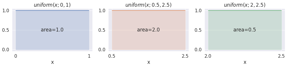
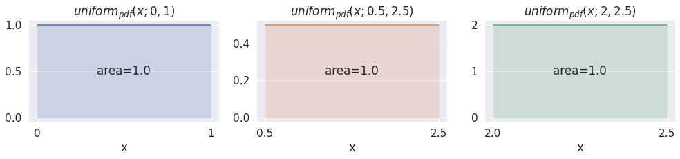
This conforms to the first requirement from above: all densities for possible values of \(x\) evaluate to a non-negative number (in this case 1.0). However, the second requirement is not fulfilled. To achieve this, all we need to do is to divide our original expression by the total area

\[ \begin{aligned} uniform_{pdf}(x; lower, upper) &= \frac{1}{\int_{lower}^{upper} 1 dx} \\ &= \frac{1}{x|_{lower}^{upper}} \\ &= \frac{1}{upper - lower} \\ \end{aligned} \]

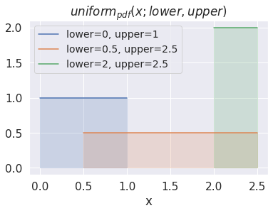
And now we have a proper uniform probability density function! It might seem like we cheated, but this is really all there is to it.

def uniform_pdf(x, lower, upper):
    return np.ones_like(x) / (upper - lower)

_, ax = plt.subplots(1, 3, figsize=(14, 3.5))

lower, upper = 0, 1
x = np.linspace(lower, upper)
plot_uniform(uniform_pdf, x, lower, upper, pdf=True, ax=ax[0], color='C0')

lower, upper = 0.5, 2.5
x = np.linspace(lower, upper)
plot_uniform(uniform_pdf, x, lower, upper, pdf=True, ax=ax[1], color='C1')

lower, upper = 2, 2.5
x = np.linspace(lower, upper)
plot_uniform(uniform_pdf, x, lower, upper, pdf=True, ax=ax[2], color='C2')

plt.tight_layout()

_, ax = plt.subplots(figsize=(6, 4))

for i, (lower, upper) in enumerate(zip((0, 0.5, 2), (1, 2.5, 2.5))):
    x = np.linspace(lower, upper)
    y = uniform_pdf(x, lower, upper)
    ax.plot(x, y, color=f'C{i}', label=f'{lower=}, {upper=}')
    ax.fill_between(x, y, color=f'C{i}', alpha=.2)

ax.set_xlabel('x')
ax.set_title('$uniform_{pdf}(x; lower, upper)$')
ax.legend(fontsize=14);

Let’s now turn to the mightier gamma distribution.

The gamma distribution #

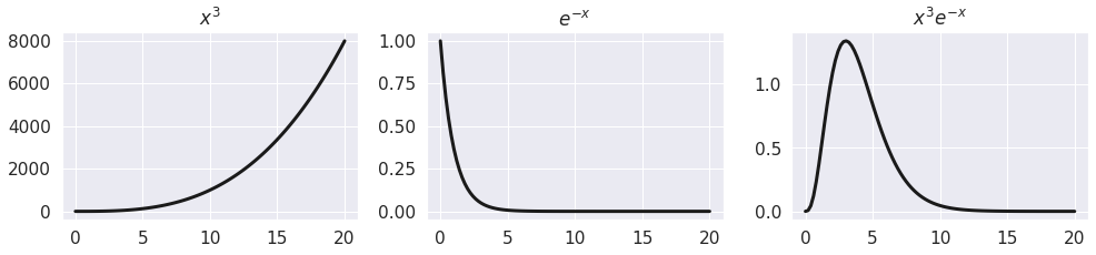
The gamma distribution is based on this funny looking function, with two parameters:

\[ gamma(x; a) = x^{a-1}e^{-x} \]

We will consider the cases where \(x > 0\) and \(a > 0\). As with the uniform, \(x\) represents the possible random outcomes, while \(a\), analogous to the \(lower\) and \(upper\), is a fixed parameter that characterizes its probability density. Unlike the uniform, this distribution is not bounded, it allows for infinitely large \(x\) outcomes.

Looking at the expression, one can notice that the first part \(x^{a-1}\) will grow quickly as x goes to \(\infty\), while the second part \(e^{-x}\) will decrease exponentially as \(x\) increases. By multiplying the two we will obtain a rising curve followed by a declining one, as the two terms change in relative importance. Here is an example with \(a=4\)

a = 4
x = np.linspace(0, 20, 100)

_, ax = plt.subplots(1, 3, figsize=(14, 3.5))

y1 = x ** (a-1)
ax[0].plot(x, y1, lw=3, color='k')
ax[0].set_title('$x^{3}$')

y2 = np.exp(-x)
ax[1].plot(x, y2, lw=3, color='k')
ax[1].set_title('$e^{-x}$')

y3 = y1 * y2
ax[2].plot(x, y3, lw=3, color='k')
ax[2].set_title('$x^{3}e^{-x}$')

plt.tight_layout()

Let’s turn it into a python function and see how the function changes with different \(a\).

def gamma(x, a):
    return x**(a-1)*np.exp(-x)    

def plot_gamma(f, x, a, ax, color, pdf=False):
    y = f(x, a)
    # Integrate area between 0 and +inf
    area_y = scipy.integrate.quad(f, 0, np.inf, args=(a,))[0]
    
    ax.plot(x, y, color=color)
    ax.fill_between(x, y, color=color, alpha=.2)
    ax.text(0.5, 0.5, f'area={area_y:.1f}', transform=ax.transAxes, ha='center', va='center')
    ax.set_xlabel('x')
    if not pdf:
        ax.set_title(f'$gamma(x; {a})$')
    else:
        ax.set_title(f'$gamma_{{pdf}}(x; {a})$')

_, ax = plt.subplots(1, 3, figsize=(14, 3.5))
x = np.linspace(0, 20, 1000)
plot_gamma(gamma, x, 4, ax=ax[0], color='C0')
plot_gamma(gamma, x, 6, ax=ax[1], color='C1')
plot_gamma(gamma, x, 8, ax=ax[2], color='C2')
plt.tight_layout()

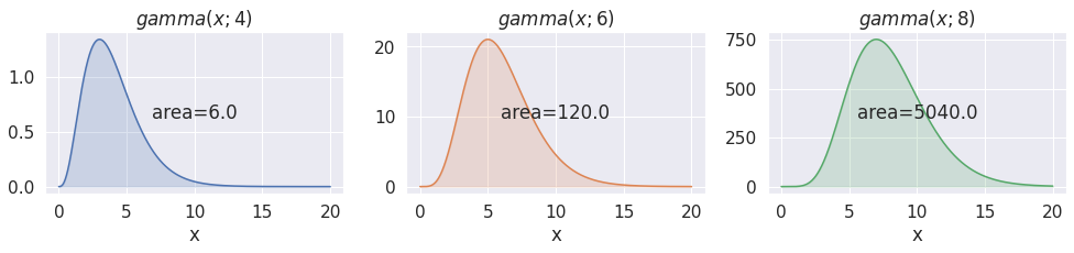
Okay, perhaps not the most amazing looking curve. But we are not looking for amazing, just nice! And there are a couple of nice things going on:

1. The function seems to be positive everywhere in the range \(x \subset [0, \infty]\)
2. It looks like the graph does not blow up as \(x\) goes to \(\infty\), even for larger \(a\)
3. The \(a\) parameter seems to have a meaningful effect on the shape of the function.

Points 1 and 2 are needed for defining an unbounded positive probability density function, while point 3 is nice for making it a useful distribution.

If you never heard about the gamma function, you might be surprised to find out that the areas for the three examples all evaluate to integer values (subject to float representation). Even more surprising is the fact that these values correspond to \((a-1)!\). And analogous to the factorial function, the area under this expression preserves a certain recursive form of \(n! = n(n-1)!\), for any positive numbers (while the factorial is only defined for integers). This surprising fact was discovered by Euler in 1730.

np.math.factorial(3), np.math.factorial(5), np.math.factorial(7)

(6, 120, 5040)

scipy.special.gamma(3.5+1), 3.5 * scipy.special.gamma(3.5)

(11.63172839656745, 11.63172839656745)

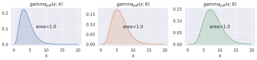
Finding the normalization constant #

In order to obtain a valid density function, we must be able to scale this function so that it integrates to 1. In theory, all we need to do is divide the original expression by the total area, as we did for the uniform.

\[ gamma_{pdf}(x; a) = \frac{x^{a-1}e^{-x}}{\int_{0}^{\infty}{x^{a-1} e^{-x} dx}} \]

However, unlike the uniform, there is no simple form for the integral in the denominator. That might be slightly annoying, but it’s not critical as long as we can compute it. In the code used to generate the plots above, I used a generic integration approximator, but, fortunately for us, some folks have found more reliable or accurate approximations that can be used to compute this integral (see the Wikipedia entries for Stirling’s and Lanczos’s approximations).

Finally, just because we cannot simplify the denominator expression, it doesn’t mean we have to write it everywhere. Let’s do some mathematical refactoring by encapsulating the denominator inside a function. To keep it math-appropriate we will use a Greek letter for its name, although something more verbose such as total_area_gamma would work as well. To keep with the convention, we will give it the uppercase gamma symbol \(\Gamma\):

\[ gamma_{pdf}(x; a) = \frac{x^{a-1}e^{-x}}{\Gamma(a)} \]

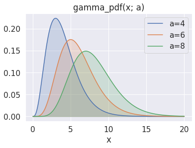
Scipy provides an implementation of the gamma function via scipy.special.gamma.

Time to plot our proper gamma density function:

def gamma_pdf(x, a):
    return x**(a-1)*np.exp(-x) / scipy.special.gamma(a) 

_, ax = plt.subplots(1, 3, figsize=(14, 3.5))
x = np.linspace(0, 20, 1000)
plot_gamma(gamma_pdf, x, 4, pdf=True, ax=ax[0], color='C0')
plot_gamma(gamma_pdf, x, 6, pdf=True, ax=ax[1], color='C1')
plot_gamma(gamma_pdf, x, 8, pdf=True, ax=ax[2], color='C2')
plt.tight_layout()

_, ax = plt.subplots(figsize=(6, 4))

x = np.linspace(0, 20, 1000)
for i, a in enumerate((4, 6, 8)):
    y = gamma_pdf(x, a)
    ax.plot(x, y, color=f'C{i}', label=f'{a=}')
    ax.fill_between(x, y, color=f'C{i}', alpha=.2)

ax.set_xlabel('x')
ax.set_title('gamma_pdf(x; a)')
ax.legend();

Adding a scale parameter #

Our pdf is neat, but can we do something more with it? Most distributions have two parameters, and we got only one: \(a\). Since more flexibility can always come in handy, why not add another one? What about adding a scaling \(b\) parameter?

According to Wikipedia, this is pretty straightforward once we have a valid pdf, which we already do:

\[ scaled_{pdf}(x, b) = \frac{1}{b}standard_{pdf}(\frac{x}{b}) \]

In our case

\[ gamma_{pdf}(x; a, b) = \frac{(\frac{x}{b})^{a-1} e^{-(\frac{x}{b})}}{b \Gamma(a)} \]

Which we can arrange as

\[ gamma_{pdf}(x; a, b) = \frac{x^{a-1} e^{-(\frac{x}{b})}}{b^{a-1}b \Gamma(a)} = \frac{x^{a-1} e^{-(\frac{x}{b})}}{b^{a} \Gamma(a)} \]

Or alternatively, we can use a precision variable \(c = \frac{1}{b}\)

\[ gamma_{pdf}(x; a, c) = \frac{c(xc)^{a-1} e^{-(xc)}}{\Gamma(a)} = \frac{c^ax^{a-1} e^{-xc}}{\Gamma(a)} \]

Let’s see what we can do with this extra parameter:

def gamma_pdf(x, a, c=1):
    return c**a * x**(a-1) * np.exp(-x*c) / scipy.special.gamma(a)

def plot_gamma_variations(a, ax, color):
    x = np.linspace(0, 20, 1000)
    base_color = seaborn.saturate(color)

    for c, saturation in zip((2, 1, 0.5), (0.8, 0.4, 0.2)):
        y = gamma_pdf(x, a=a, c=c)
        color = seaborn.desaturate(base_color, saturation)
        ax.plot(x, y, color=color, label=f'{c=}')
        ax.fill_between(x, y, color=color, alpha=.2)

    ax.set_xlabel('x')
    ax.set_title(f'$gamma_{{pdf}}(x;{a},c)$')
    ax.legend()

_, ax = plt.subplots(1, 3, figsize=(14, 3.5))
plot_gamma_variations(a=4, ax=ax[0], color='C0')
plot_gamma_variations(a=6, ax=ax[1], color='C1')
plot_gamma_variations(a=8, ax=ax[2], color='C2')
plt.tight_layout()

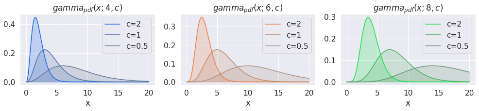
The parameter names \(a\), \(b\), and \(c\), deviate from traditional characterizations of the gamma distribution. Wikipedia, for example, uses \(k\) and \(\theta\) for our \(a\) and scale \(b\), and a distinct pair of parameter names \(\alpha\) and \(\beta\) for our \(a\) and precision \(c\) parameterization. \(\lambda\) is also commonly used for the precision parameter, as this is linked conceptually to the exponential \(\lambda\) rate parameter. Speaking of which, “rate” is an alternative, and perhaps more common name, for “precision”.

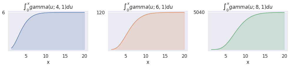
Bonus: deriving the CDF of the gamma distribution #

We got the gamma pdf, let’s get the cumulative distribution function (CDF) as well. Recall that the CDF of a distribution \(X\) is the matematical function that returns the \(P(X<=x)\), that is the probability that the random \(x\) value is lower or equal to a specific number. Since it defines an interval, in our case \([0, x]\), it is appropriate to talk about probabilities and not just densities.

\[ gamma\_cdf(x; a, c) = \frac{\int_0^x c^a(u)^{a-1} e^{-(cu)} du}{\Gamma(a)}\]

Note that we need a new variable \(u\) to distinguish the limit of integration from the integrand. Also, for the very same reason as before, the \(\Gamma(a)\) is there to make sure the CDF evaluates to \(1\) when \(x=\infty\)

This article would have been slightly less unrealistic if it had started with the derivation of the CDF, since the Gamma integral function is what actually came down to us through history.

def plot_gamma_integral(a, ax, color, cdf=False):
    x = np.logspace(0.1, 1.3)
    y = scipy.special.gammainc(a, x)
    assymptote = 1
    # gammainc returns the already normalized incomplete integral
    gamma = scipy.special.gamma(a)
    y *= gamma
    
    ax.plot(x, y, color=color)
    ax.fill_between(x, y, color=color, alpha=.2)
    ax.set_yticks([gamma])
    ax.grid(None, axis='x')
    ax.set_xlabel('x')
    
    ax.set_title(f'$\int_0^{{x}}gamma(u; {a}, 1) du$')

_, ax = plt.subplots(1, 3, figsize=(14, 3.5))
plot_gamma_integral(4, ax=ax[0], color='C0')
plot_gamma_integral(6, ax=ax[1], color='C1')
plot_gamma_integral(8, ax=ax[2], color='C2')
plt.tight_layout()

_, ax = plt.subplots(figsize=(6, 4))

x = np.logspace(0.1, 1.3)
for i, a in enumerate((4, 6, 8)):
    y = scipy.special.gammainc(a, x)
    ax.plot(x, y, color=f'C{i}', label=f'{a=}')
    ax.fill_between(x, y, color=f'C{i}', alpha=.2)

ax.set_xlabel('x')
ax.set_title(f'$gamma_{{cdf}}(x; a, 1)$')
ax.legend();

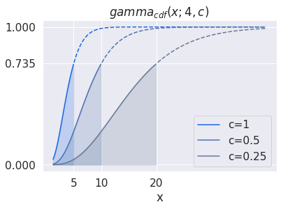
The CDF expression can be further simplified with a change of variables \(t = cu\) \[ \begin{aligned} gamma\_cdf(x; a, c) &= \frac{\int_0^x c^a(u)^{a-1} e^{-(cu)} du}{\Gamma(a)} \\ &= \frac{1}{\Gamma(a)} \int_0^x c(cu)^{a-1} e^{-(cu)} du \\ &= \frac{1}{\Gamma(a)} \int_0^{xc} c(t)^{a-1} e^{-t} \frac{1}{c}dt \quad \begin{cases} \text{change of variables} \\ t = cu \\ dt = c\,du \\ \frac{1}{c}dt = du \\ \end{cases} \\ &= \frac{1}{\Gamma(a)} \int_0^{xc} t^{a-1} e^{-t} dt \end{aligned} \]

Which reveals that the inverse scaling by \(c\) has an effect on increasing or reducing the area of a standard gamma distribution that is contained below \(x\)

_, ax = plt.subplots(figsize=(6, 4))
x = np.logspace(0.1, 1.6, 200)

base_color = seaborn.saturate('C0')
cutoff = 5

for c, saturation in zip(
    (1, 0.5, 0.25),
    (0.8, 0.4, 0.2)
):
    color = seaborn.desaturate(base_color, saturation)
    where = x<=(cutoff/c)
    
    y = scipy.special.gammainc(4, x*c)
    ax.plot(x[where], y[where], color=color, label=f'{c=}')
    ax.plot(x[~where], y[~where], color=color, ls='--')
    ax.fill_between(x, y, where=where, color=color, alpha=.2)

ax.set_xticks([5, 10, 20])
ax.set_yticks([0, scipy.special.gammainc(4, cutoff), 1])
ax.set_xlabel('x')
ax.set_title(f'$gamma_{{cdf}}(x; 4, c)$')
# ax.set_ylabel(r'$\frac{\int_0^{xc}{f(a, u)} du}{area\_f(x)}$')
ax.legend();

Similar to what we did with the pdf, it’s common to refactor the numerator integral expression into its own function. This is called lower incomplete gamma function, or more succintly the lower case gamma \(\gamma\) letter. \[ gamma\_cdf(x; a, c) = \frac{\int_0^{xc} t^{a-1} e^{-t} dt}{\Gamma(a)} = \frac{\gamma(a, xc)}{\Gamma(a)} \]

As with the gamma function, there are quick and stable numerical implementations of the incomplete gamma function. In scipy this can be obtained by scipy.special.gammainc(a, x) * scipy.special.gamma(a). The multiplication is needed because the default scipy.special.gammainc already contains the \(gamma(a)\) normalization term.

Similarly to the gamma distribution, which gets its name from the gamma integral function \(\Gamma\), the beta distribution also gets its name from the beta integral function \(B\). In fact the two distributions are closely related.