Derivatives, integrals, anti-derivatives and anti-integrals
April 10, 2022
import numpy as np
import matplotlib.pyplot as plt
import seaborn
seaborn.set_style('darkgrid')
seaborn.set(font_scale=1.2)
def draw_arrows(ax, top_from, top_to, top_text_xy, bottom_from, bottom_to, bottom_text_xy, diff_top=True):
    text_top = "Differentiation"
    text_bottom = "Integration"
    if not diff_top:
        text_top, text_bottom = text_bottom, text_top

    ax.annotate(
        "", top_from, top_to,
        xycoords="axes fraction",
        size="large", ha="left", va="center",
        arrowprops=dict(
            arrowstyle="->", color="k", lw=2,
            connectionstyle="angle3,angleA=50,angleB=-50",
        ),
    )

    ax.text(*top_text_xy, text_top, transform=ax.transAxes, ha="center")

    ax.annotate(
        "", bottom_from, bottom_to,
        xycoords="axes fraction",
        size="large", ha="left", va="center",
        arrowprops=dict(
            arrowstyle="->", color="k", lw=2,
            connectionstyle="angle3,angleA=50,angleB=-50",
        ),
    )
    ax.text(*bottom_text_xy, text_bottom, transform=ax.transAxes, ha="center")

def draw_deltas(ax, dx_from, dx_to, dx_width, dy_from, dy_to, dy_width, y_is_delta=True):
    ax.annotate(
        "$\Delta x$", dx_from, dx_to,
        size="large", ha="center", va="center",
        arrowprops=dict(arrowstyle=f"-[, widthB={dx_width}", color="k",),
    )
    ax.annotate(
        "$\Delta y$" if y_is_delta else "$y$", dy_from, dy_to,
        size="large", ha="left", va="center",
        arrowprops=dict(arrowstyle=f"-[, widthB={dy_width}", color="k"),
    )
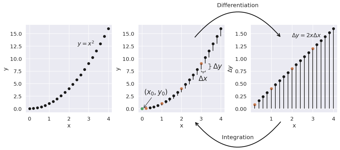
There are two ways of describing a sequence of (\(x\), \(y\)) points:
- Enumerate all (\(x\), \(y\)) pairs
- Specify the first (\(x_0\), \(y_0\)) pair and the distance (\(\Delta x\), \(\Delta y\)) of each subsequent point
In a loose sense, differentiation goes from 1. to 2., and integration goes from 2. to 1.
f = lambda x: x ** 2
df = lambda x: 2 * x

dx = 0.2
x = np.arange(0, 4+dx, dx)
y = f(x)
focus = np.array([1, 5, 10, 15])

fig, axes = plt.subplots(1, 3, figsize=(14, 4))
fig.subplots_adjust(wspace=0.3)

ax = axes[0]
ax.scatter(x, y, color="k")
ax.text(3.5-0.2, f(3.5), "$y = x^2$", va="bottom", ha="right")
ax.set_ylabel("y")

ax = axes[1]
ax.scatter(x, y, color="k")
ax.scatter(x[0], y[0], color="C2")
ax.scatter(x[focus], y[focus], color="C1")
ax.vlines(x[1:], y[:-1], y[1:], color="k")
ax.annotate(
    "$(x_0, y_0)$", (0.05, -0.05), (.1, 3.3),
    size="large", ha="left", va="center",
    arrowprops=dict(arrowstyle="->", color="k"),
)
ax.set_ylabel("y")

mid = (f(3-dx) + f(3)) / 2
draw_deltas(
    ax,
    (3 + dx/2, 7.5), (3 + dx/2, 6), 0.3,
    (3 + dx*2, mid), (3 + 0.6, mid), 0.4
)

ax = axes[2]
ax.scatter(x[1:], df(x)[1:] * dx, color="k")
ax.scatter(x[focus], df(x)[1:][focus-1] * dx, color="C1")
ax.vlines(x[1:], 0, df(x)[1:] * dx, color="k")
ax.text(3.5-0.1, df(3.5) * dx, "$\Delta y = 2x \Delta x$", va="bottom", ha="right")
ax.set_ylabel("$\Delta y$")

draw_arrows(
    ax,
    (0.35, 0.85), (-0.65, 0.85), (-0.15, 1.2),
    (-0.65, -0.1), (0.35, -0.1), (-0.15, -.3),
)

for ax in axes:
    ax.set_xlabel("x")
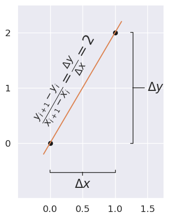
Actually when we differentiate, we rather store the ratio of \(\frac{\Delta y}{\Delta x}\), which is also the slope of the straigth line that connects \((x_i, y_i)\) to \((x_{i+1}, y_{i+1})\)
fig, ax = plt.subplots(figsize=(4.5/1.2,6/1.2))
ax.scatter([0, 1], [0, 2], c="k")
ax.plot([-0.1, 1.1], [-0.2, 2.2], c="C1")

plt.text(
    0.25, 1.15,
    "$\\frac{y_{i+1} - y_i}{x_{i+1} - x_i} = \\frac{\Delta y}{\Delta x} = 2$",
    ha="center", va="center", fontsize=20,
    rotation=60.5,
)

ax.annotate(
    "$\Delta x$", (0.5, -0.5), (0.5, -0.75),
    size="large", ha="center", va="center",
    arrowprops=dict(arrowstyle="-[, widthB=2.7", color="k",),
)

ax.set_ylim([-1, 2.5])
ax.set_xlim([-0.5, 1.75])
ax.annotate(
    "$\Delta y$", (1.25, 1.0), (1.5, 1.0),
    size="large", ha="left", va="center",
    arrowprops=dict(arrowstyle="-[, widthB=4.6", color="k"),
)

ax.set_xticks([0, 0.5, 1, 1.5])
ax.set_yticks([0, 1, 2]);
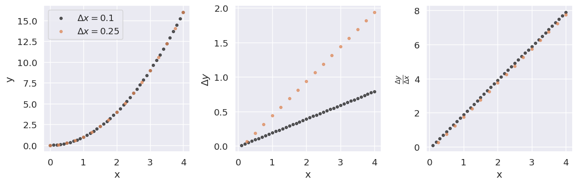
This makes it so that the output of differentation is mostly the same regardless of the density of points in the original curve
dx1 = 0.1
x1 = np.arange(0, 4+dx1, dx1)

dx2 = 0.25
x2 = np.arange(0, 4+dx2, dx2)
fig, axes = plt.subplots(1, 3, figsize=(12, 4))

ax = axes[0]
ax.scatter(x1, f(x1), color="k", alpha=0.7, s=14, label=f"$\Delta x = {dx1}$")
ax.scatter(x2, f(x2), color="C1", alpha=0.7, s=14, label=f"$\Delta x = {dx2}$")
ax.legend()
ax.set_ylabel("y")
ax.set_xlabel("x")

ax = axes[1]
ax.scatter(x1[1:], np.diff(f(x1)), color="k", alpha=0.7, s=14)
ax.scatter(x2[1:], np.diff(f(x2)), color="C1", alpha=0.7, s=14)
ax.set_ylabel("$\Delta y$")
ax.set_xlabel("x")

ax = axes[2]
ax.scatter(x1[1:], np.diff(f(x1)) / dx1, color="k", alpha=0.7, s=14)
ax.scatter(x2[1:], np.diff(f(x2)) / dx2, color="C1", alpha=0.7, s=14)
ax.set_ylabel("$\\frac{\Delta y}{\Delta x}$")
ax.set_xlabel("x")

fig.tight_layout();
Integration as the inverse of differentation #
Once we have a set of differences (or difference ratios), we can restore the original curve by adding those differences, starting from the initial point \((x0, y0)\)
\[y_i = y_0 + \sum_0^x{\Delta y_i} = y_0 + \sum_0^x{\frac{\Delta y_i}{\Delta x}}\Delta x\]
fig, axes = plt.subplots(1, 3, figsize=(12, 4))

ax = axes[0]
ax.scatter(x1[1:], np.diff(f(x1)) / dx1, color="k", alpha=0.7, s=14, label=f"$\Delta x = {dx1}$")
ax.scatter(x2[1:], np.diff(f(x2)) / dx2, color="C1", alpha=0.7, s=14, label=f"$\Delta x = {dx2}$")
ax.legend();
ax.set_ylabel("$\\frac{\Delta y}{\Delta x}$")

ax = axes[1]
ax.scatter(x1, np.cumsum(np.diff(f(x1), prepend=x1[0]) / dx1), color="k", alpha=0.7, s=14)
ax.scatter(x2, np.cumsum(np.diff(f(x2), prepend=x2[0]) / dx2), color="C1", alpha=0.7, s=14)

ax = axes[1]
ax.scatter(x1, np.cumsum(np.diff(f(x1), prepend=x1[0]) / dx1), color="k", alpha=0.7, s=14)
ax.scatter(x2, np.cumsum(np.diff(f(x2), prepend=x2[0]) / dx2), color="C1", alpha=0.7, s=14)
ax.set_ylabel("$y_0 + \sum_0^x{\\frac{\Delta y}{\Delta x}}$")

ax = axes[2]
ax.scatter(x1, np.cumsum(np.diff(f(x1), prepend=x1[0]) / dx1) * dx1, color="k", alpha=0.7, s=14)
ax.scatter(x2, np.cumsum(np.diff(f(x2), prepend=x2[0]) / dx2) * dx2, color="C1", alpha=0.7, s=14)
ax.set_ylabel("$y_0 + \sum_0^x{\\frac{\Delta y}{\Delta x}\Delta x} = y_0 + \sum_0^x{\Delta y}$")

for ax in axes:
    ax.set_xlabel("x")

fig.tight_layout();
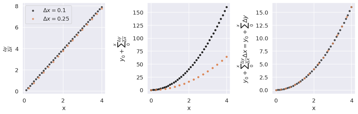
In that sense integration is the inverse of differentation in the same sense that addition and multiplication are the inverses of subtraction and division.
If we add up (integrate) all the differences from a starting point, we get back the original series.
But this process of integration has another interesting meaning…
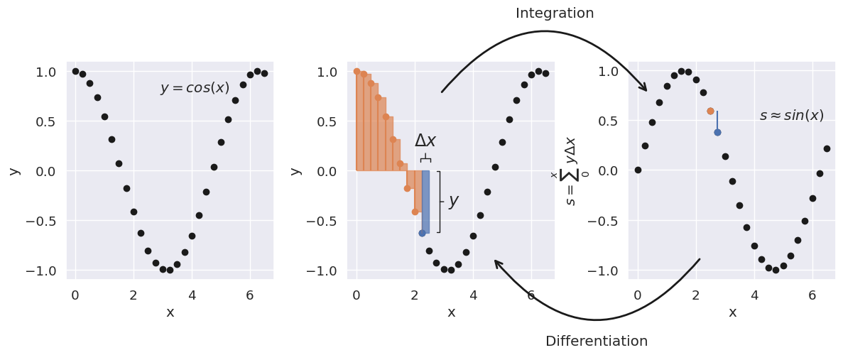
Differentiation as the inverse of integration #
Let’s grab the leftmost plot from above and forget that it describes \(\frac{\Delta y}{\Delta x}\).
Let’s say we have just a vanilla \(y = 2x\) series.
What are we doing when we add up all the \(y\) up to \(x\) and multiply by \(\Delta x\)?
\[s_i = \sum_0^x{y \Delta x}\]
g = lambda x : 2*x
sg = lambda x : x ** 2

dx = 0.25
x = np.arange(0, 3.5+dx, dx)
y = g(x)
focus = 9

fig, axes = plt.subplots(1, 3, figsize=(14, 4))
fig.subplots_adjust(wspace=0.3)

ax = axes[0]
ax.scatter(x, y, color="k")
ax.text(3.2-0.2, g(3.2), "$y = 2x$", va="bottom", ha="right")
ax.set_ylabel("y")

ax = axes[1]
ax.scatter(x[focus:], y[focus:], color="k")
ax.scatter(x[:focus], y[:focus], color="C1")
ax.scatter(x[focus], y[focus], color="C0")
ax.vlines(x[:focus], 0, y[:focus], color="C1")
ax.fill_between(x[:focus+1], 0, y[:focus+1], step="post", color="C1", alpha=0.7)
ax.bar(x[focus]+dx/2, y[focus], width=dx, color="C0", alpha=0.7, ec="C0")
ax.set_ylabel("y")
ax.set_ylim([-.5, None])
mid = y[focus] / 2
draw_deltas(
    ax,
    (x[focus] + dx/2, y[focus] + 1.0), (x[focus] + dx/2, y[focus] + 1.8), 0.4,
    (x[focus] + dx + 0.15, mid), (x[focus] + dx + 0.4, mid), 3.58,
    y_is_delta=False,
)

ax = axes[2]
ax.scatter(x, sg(x), color="k")
ax.scatter(x[focus-1], sg(x[focus-1]), color="C1")
ax.scatter(x[focus], sg(x[focus]), color="C0")
ax.vlines(x[focus], sg(x[focus-1]), sg(x[focus]), color="C0")
ax.text(3.1 - 0.2, sg(3.1), "$s \\approx x^2$", ha="right")
ax.set_ylabel("$s = \sum_0^x{\ y \Delta x}$", labelpad=-5)

draw_arrows(
    ax,
    (0.35-0.2, 0.85), (-0.65-0.2, 0.85), (-0.15, 1.2),
    (-0.65, -0.1), (0.35, -0.1), (-0.15, -.3),
    diff_top=False,
)

for ax in axes:
    ax.set_xlabel("x")
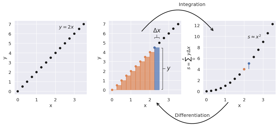
We are adding up the areas of the rectangles below \(y\) up to \(x\)! So our function \(s\) is an area function!
Now, the difference between successive points in that area function \(\Delta s_i\) gives us the difference in areas up to \(x_{i}\) and up to \(x_{i-1}\), which must intuitively be \(y_i\Delta x\) and the ratio \(\frac{y_i \Delta x}{\Delta x} = y_i\)
This is just another way of saying that differentation is the inverse of integration.
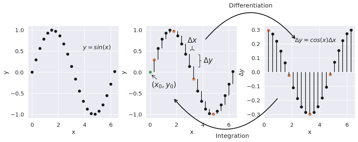
Bonus: Illustrating the sin function #
f = lambda x: np.sin(x)
df = lambda x: np.cos(x)

dx = 0.3
x = np.arange(0, np.pi*2+dx, dx)
y = f(x)
focus = np.array([1, 6, 11, 16])

fig, axes = plt.subplots(1, 3, figsize=(14, 4))
fig.subplots_adjust(wspace=0.3)

ax = axes[0]
ax.scatter(x, y, color="k")
ax.text(6, 0.5, "$y = sin(x)$", va="bottom", ha="right")
ax.set_ylabel("y")

ax = axes[1]
ax.scatter(x, y, color="k")
ax.scatter(x[0], y[0], color="C2")
ax.scatter(x[focus], y[focus], color="C1")
ax.vlines(x[1:], y[:-1], y[1:], color="k")
ax.annotate(
    "$(x_0, y_0)$", (0.05, -0.05), (.1, -.3),
    size="large", ha="left", va="center",
    arrowprops=dict(arrowstyle="->", color="k"),
)
draw_deltas(
    ax,
    (3.2, 0.52), (3.2, 0.75), .25,
    (3.7, 0.27), (4.05, 0.27), .85,
)
ax.set_ylabel("y")

ax = axes[2]
ax.scatter(x[1:], np.diff(y), color="k")
ax.scatter(x[focus], np.diff(y)[focus-1], color="C1")
ax.vlines(x[1:], 0, np.diff(y), color="k")
ax.text(5.25, 0.2, "$\Delta y \\approx cos(x) \Delta x$", va="bottom", ha="right")
ax.set_ylabel("$\Delta y$")

draw_arrows(
    ax,
    (0.35, 0.85), (-0.65, 0.85), (-0.15, 1.2),
    (-1.0, 0.22), (0.15, 0.22), (-0.35, -.21),
)

for ax in axes:
    ax.set_xlabel("x");
g = lambda x : np.cos(x)
sg = lambda x : np.sin(x)

dx = 0.25
x = np.arange(0, np.pi*2+dx, dx)
y = g(x)
focus = 9

fig, axes = plt.subplots(1, 3, figsize=(14, 4))
fig.subplots_adjust(wspace=0.35)

ax = axes[0]
ax.scatter(x, y, color="k")
ax.text(5.3, 0.75, "$y = cos(x)$", va="bottom", ha="right")
ax.set_ylabel("y")

ax = axes[1]
ax.scatter(x[focus:], y[focus:], color="k")
ax.scatter(x[:focus], y[:focus], color="C1")
ax.scatter(x[focus], y[focus], color="C0")
ax.vlines(x[:focus], 0, y[:focus], color="C1")
ax.fill_between(x[:focus+1], 0, y[:focus+1], step="post", color="C1", alpha=0.7)
ax.bar(x[focus]+dx/2, y[focus], width=dx, color="C0", alpha=0.7, ec="C0")
ax.set_ylabel("y")
# ax.set_ylim([-.5, None])
mid = y[focus] / 2
draw_deltas(
    ax,
    (x[focus] + dx/2, 0.1), (x[focus] + dx/2, .3), 0.3,
    (x[focus] + dx + 0.3, mid), (x[focus] + dx + 0.65, mid), 1.78,
    y_is_delta=False,
)

ax = axes[2]
ax.scatter(x, sg(x), color="k")
ax.scatter(x[10], sg(x[10]), color="C1")
ax.scatter(x[11], sg(x[11]), color="C0")
ax.vlines(x[11], sg(x[10]), sg(x[11]), color="C0")
ax.text(6.5 - 0.1, sg(6.5)+ 0.3, "$s \\approx sin(x)$", ha="right")
ax.set_ylabel("$s = \sum_0^x{\ y \Delta x}$", labelpad=-5)

draw_arrows(
    ax,
    (0.35-0.25, 0.85), (-0.65-0.25, 0.85), (-0.35, 1.2),
    (-0.65, .1), (0.35, 0.1), (-0.15, -.3),
    diff_top=False,
)

for ax in axes:
    ax.set_xlabel("x")