A simple Sequential Monte Carlo algorithm for posterior approximation
August 6, 2021
Introduction #
Sequential Monte Carlo (SMC) can be used to take samples from posterior distributions, as an alternative to popular methods such as Markov Chain Monte Carlo (MCMC) like Metropolis-Hastings, Gibbs Sampling or more state-of-the-art Hamiltonian Monte Carlo (HMC) and No-U-Turn Sampler (NUTS).
Instead of creating a single Markov Chain, SMC works by keeping track of a large population of samples, which, in a similar spirit to Genetic Algorithms can be “selected” and “mutated” to evolve a better “fit” to the posterior distribution.
Experience suggests SMC is particularly well fit to the following settings:
- Multi-modal posterior distributions
- Online inference when data accumulates over time
- Approximate Bayesian Inference when the likelihood function cannot be easily written down
In this article I introduce the basic components that make up a simple SMC algorithm. In future articles, I present more complex variations that build up towards the specific algorithm that is employed in the PyMC3 library.
Toy 2D Gaussian example #
As with MCMC, SMC approximates the posterior distribution via careful weighted sampling. However, while MCMC approximates a distribution through a single random walk that unrolls over time, SMC does this in a parallel manner. At each step, it keeps track of a series of samples (also known as particles) that approximate the distribution as a whole.
This picture tries to illustrate this distinction for a simple 2D Gaussian posterior that will be used throughout this article:
\(\)
\[ \text{pdf}(x, y) = \text{exp}(-\begin{bmatrix}x\\ y\end{bmatrix}^T \begin{bmatrix}1&0.5\\ 0.5&1\end{bmatrix}^{-1} \begin{bmatrix}x\\ y\end{bmatrix}) \]
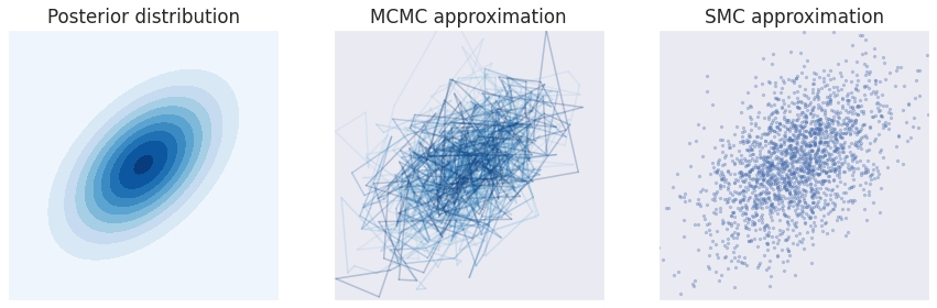
Approximation to the 2D Gaussian posterior shown on the left plot. The middle plot shows the approximation from a single MCMC chain, with the samples connected sequentially, emphasizing the autocorrelated random walk behavior. The right plot shows the approximation from the SMC algorithm, where each sample is independent from the rest.
Why are we even doing this?
The example above with a 2D Gaussian is deceptively simple and there is no reason why we would need to use Monte Carlo approximations (be it MCMC or SMC) to understand it. Usually in the context of Bayesian data analysis we are working with a model that describes a complicated and highly dimensional posterior distribution that cannot be written down mathematically (or as mathematicians prefer, analytically).
In addition, even if the posterior distribution could be described mathematically, it is often very difficult to work with. We are usually interested in chopping the posterior distribution into a smaller number of components that we care about (marginalization) or summarizing it into metrics that are understandable such as correlations, averages and standard deviations (expectations). Surprisingly, these sort of operations are trivial if we can get a hold of a representative set of samples from the distribution in question. All we need is to do some smart indexing and call functions such as
numpy.mean()andnumpy.std()!
The core of the SMC algorithm is very simple:
- We start by creating a large population of particles, usually by sampling from the prior distribution.
- We then compute a weight for each particle, which is proportional to the posterior probability at that “point”.
- These weights are used to sample, with replacement, a new population of particles. This will lead to a population that is more representative of the posterior distribution. On average, a particle that is 3x more probable than another will be resampled 3x as often.
- Finally, we introduce some “mutations” in the population. This could be as simple as adding a random uniform jittering to each particle dimension, but, we can also try to “guide” the particles in a more clever way towards areas of larger posterior mass.
The pseudocode for the SMC algorithm is given below:
# hyperparameters
n_particles = 2000
n_steps = 10

# initialize population of particles from prior
particles = sample_prior(n_particles)
# main loop
for step in range(n_steps):
    # compute particle weights in proportion
    # to the posterior distribution probability
    weights = compute_weights(particles, posterior)
    # resample particles (with replacement)
    # based on their weights
    particles = resample(particles, weights)
    # mutate particles to reintroduce variation
    # and better explore the posterior distribution
    particles = mutate(particles)
# final approximation is given by the final particles
posterior = particles
Let’s flesh out these steps in detail.
A particle is born #
What is a particle?
A particle (or a sample in conventional MCMC) is a numerical vector with one entry for each parameter in the posterior function that we are interested in. In the 2D Gaussian example above it was a 2D-vector with
{x, y}coordinates.particle = {"x": -0.5, "y": 0.2}In a simple linear regression model it might be an \(N^D\)-vector containing a value for the
intercept, acoefficientfor each predictor in our dataset and anoiseterm for the observations.particle = {"intercept": 1.0, "coef_1": 0.5, "coef_2": 0.2, "noise": 3.0}
import numpy as np
import scipy.stats as st
import matplotlib.pyplot as plt
import seaborn as sns
sns.set_style("dark")
sns.set(font_scale = 1.4)
def create_plot(rows=1, cols=1):
    fig, ax = plt.subplots(rows, cols, figsize=(6*cols, 6*rows), sharex=True, sharey=True)

    # single plot
    if rows + cols == 2:
        ax.set_aspect('equal', 'box')
        ax.set_xticks([])
        ax.set_yticks([])

    # multiple plot
    else:
        for axi in ax.ravel():
            axi.set_aspect('equal', 'box')
            axi.set_xticks([])
            axi.set_yticks([])

    return fig, ax
def make_arrow(a, b, axA, axB):
    from matplotlib.patches import ConnectionPatch

    return ConnectionPatch(
        a,
        b,
        coordsA="axes fraction",
        coordsB="axes fraction",
        axesA=axA,
        axesB=axB,
        color="k",
        fc="k",
        arrowstyle="-|>",
        mutation_scale=30,
        lw=2,
        zorder=10,
    )
Let’s create our very first particles:
class Particle:
    def __init__(self, x, y):
        self.x = x
        self.y = y

adam, eve = Particle(x=1, y=0), Particle(x=0, y=1)
_, ax = create_plot()
ax.scatter(adam.x, adam.y)
ax.annotate("Adam", (adam.x, adam.y+.1), ha="center", fontsize=16)
ax.scatter(eve.x, eve.y)
ax.annotate("Eve", (eve.x, eve.y+.1), ha="center", fontsize=16)
ax.set_xlim([-0.5, 1.5])
ax.set_ylim([-0.5, 1.5]);
Kidding aside, we need to get a whole population of particles. How should we choose?
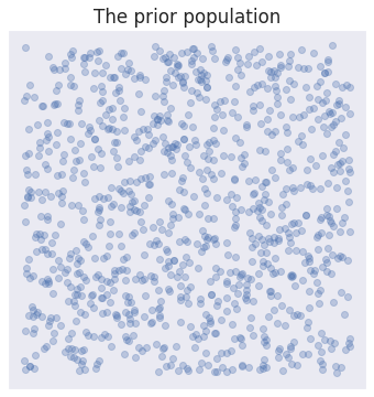
Making the effort to pick a good initial population can be very useful. Remember that the goal is to obtain a representative sample from the posterior distribution, and so the closer our initial population is to the posterior, the closer we are to being done.
Regardless, and to keep things simple with our toy example, we will just take a random sample from the uniform grid:
def sample_uniform_grid(min_x, max_x, min_y, max_y, n):
    particles = []
    for i in range(n):
        x = np.random.uniform(min_x, max_x)
        y = np.random.uniform(min_y, max_y)
        particle = Particle(x=x, y=y)
        particles.append(particle)
    return particles
particles = sample_uniform_grid(-3, 3, -3, 3, n=1000)
xs = [particle.x for particle in particles]
ys = [particle.y for particle in particles]

_, ax = create_plot()
ax.scatter(xs, ys, alpha=0.3)
ax.set_title("The prior population");
Picking favorites #
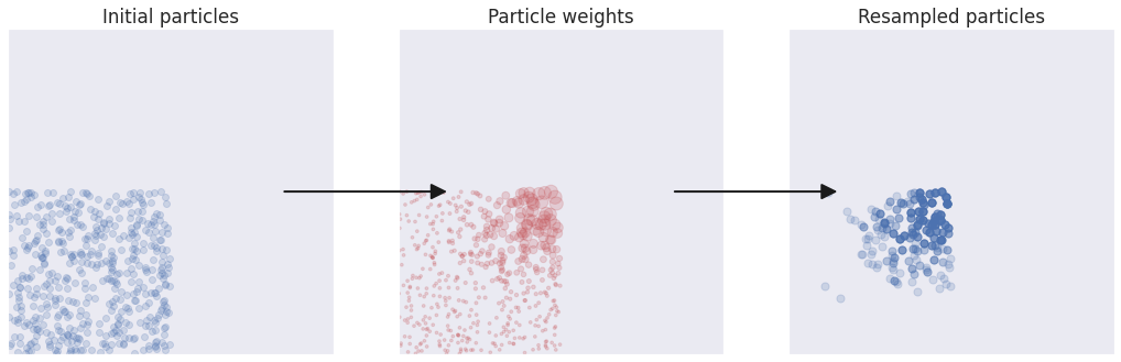
Now that we have a population of particles, it’s time to evolve it into a proper approximation of the posterior distribution! To do this, we weight each particle by its posterior probability, normalize all the population weights so that they add up to 1.0 and use them to resample with replacement.
def posterior(particle):
    """
    Unnormalized 2D Gaussian with [0, 0] mean
    and [[0.5, 1.0], [1.0, 0.5]] covariance matrix
    """
    xy = np.array([particle.x, particle.y])
    cov = np.array([[1.0, 0.5], [0.5, 1.0]])
    return np.exp(-(xy) @ np.linalg.inv(cov) @ (xy))
def compute_weights(particles, posterior):
    weights = np.array([posterior(particle) for particle in particles])
    weights /= np.sum(weights)  # normalize weights
    return weights
def resample(particles, weights):
    idxs = np.arange(len(particles))
    sampled_idxs = np.random.choice(idxs, p=weights, replace=True, size=len(particles))
    resampled_particles = []
    for idx in sampled_idxs:
        resampled_particles.append(particles[idx])
    return resampled_particles
_, ax = create_plot(1, 3)

xs = [particle.x for particle in particles]
ys = [particle.y for particle in particles]
ax[0].scatter(xs, ys, alpha=0.2)
ax[0].set_title("Initial particles")

weights = compute_weights(particles, posterior)
rescaled_weights = 0.95 * (weights - np.min(weights)) / (np.max(weights) - np.min(weights)) + 0.05
ax[1].scatter(xs, ys, s=150 * rescaled_weights, alpha=0.2, color="C3")
ax[1].set_title("Particle weights")

resampled_particles = resample(particles, weights)
xs = [particle.x for particle in resampled_particles]
ys = [particle.y for particle in resampled_particles]
ax[2].scatter(xs, ys, s=50, alpha=0.2)
ax[2].set_title("Resampled particles")

ax[1].add_artist(make_arrow((0.85, 0.5), (0.15, 0.5), ax[0], ax[1]));
ax[2].add_artist(make_arrow((0.85, 0.5), (0.15, 0.5), ax[1], ax[2]));
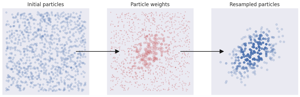
The initial population of particles is shown on the left plot. In the middle plot each particle is given a weight proportional to its posterior probability. The weights are illustrated by the particle size. In the right plot, the particles were resampled with replacement based on their weights. Each particle is plotted with the same transparency, and those resampled multiple times appear to be darker.
Introducing variation #
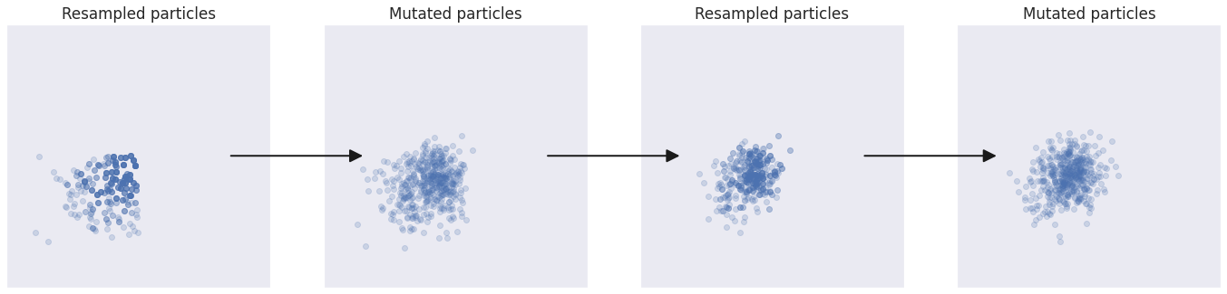
The example above was a favorable one, where the initial population of particles happened to cover the bulk of the posterior distribution. We may not always be this lucky, for instance when working with very complex distributions or when our choice for initial population of particles is not great, as in the exaggerated example below:
_, ax = create_plot(1, 3)
ax[0].set_xlim([-3, 3])
ax[0].set_ylim([-3, 3])

bad_particles = sample_uniform_grid(-3, 0, -3, 0, 500)
xs = [particle.x for particle in bad_particles]
ys = [particle.y for particle in bad_particles]
ax[0].scatter(xs, ys, alpha=0.2)
ax[0].set_title("Initial particles")

weights = compute_weights(bad_particles, posterior)
rescaled_weights = 0.95 * (weights - np.min(weights)) / (np.max(weights) - np.min(weights)) + 0.05
ax[1].scatter(xs, ys, s=150 * rescaled_weights, alpha=0.2, color="C3")
ax[1].set_title("Particle weights")

bad_resampled_particles = resample(bad_particles, weights)
xs = [particle.x for particle in bad_resampled_particles]
ys = [particle.y for particle in bad_resampled_particles]
ax[2].scatter(xs, ys, s=50, alpha=0.2)
ax[2].set_title("Resampled particles")

ax[1].add_artist(make_arrow((0.85, 0.5), (0.15, 0.5), ax[0], ax[1]));
ax[2].add_artist(make_arrow((0.85, 0.5), (0.15, 0.5), ax[1], ax[2]));
To obtain a robust algorithm we need some way for the population to “evolve” towards the target distribution. This is achieved by mutating the particles.
The mutation step is also important for reintroducing variability after the resampling step. Because resampled particles are exact copies of each other, if we were to rerun the weighting and resampling steps several times, the population would quickly converge to a singular particle.
Blind evolution #
The simplest mutation strategy is to add a random offset to each particle parameter:
def random_mutation(particles):
    new_particles = []
    for particle in particles:
        # Add Gaussian noise around each particle dimension
        new_x = particle.x + np.random.normal(0, .2)
        new_y = particle.y + np.random.normal(0, .2)
        new_particle = Particle(x=new_x, y=new_y)
        new_particles.append(new_particle)
    return new_particles
_, ax = create_plot(1, 4)
ax[0].set_xlim([-3, 3])
ax[0].set_ylim([-3, 3])

particles = bad_resampled_particles
xs = [particle.x for particle in particles]
ys = [particle.y for particle in particles]
ax[0].scatter(xs, ys, alpha=0.2)
ax[0].set_title("Resampled particles")

particles = random_mutation(particles)
new_xs = [particle.x for particle in particles]
new_ys = [particle.y for particle in particles]
ax[1].scatter(new_xs, new_ys, alpha=0.2)
ax[1].set_title("Mutated particles")

weights = compute_weights(particles, posterior)
particles = resample(particles, weights)
xs = [particle.x for particle in particles]
ys = [particle.y for particle in particles]
ax[2].scatter(xs, ys, alpha=0.2)
ax[2].set_title("Resampled particles")

particles = random_mutation(particles)
new_xs = [particle.x for particle in particles]
new_ys = [particle.y for particle in particles]
ax[3].scatter(new_xs, new_ys, alpha=0.2)
ax[3].set_title("Mutated particles")

ax[1].add_artist(make_arrow((0.85, 0.5), (0.15, 0.5), ax[0], ax[1]));
ax[2].add_artist(make_arrow((0.85, 0.5), (0.15, 0.5), ax[1], ax[2]));
ax[3].add_artist(make_arrow((0.85, 0.5), (0.15, 0.5), ax[2], ax[3]));
Intelligent design #
Creationists might have gotten it wrong when it comes to natural selection, but their premise makes a lot of sense: It would all have been much easier if someone had taken the driving seat. Fortunately that is something we can do in SMC, and in particular when it comes to how we mutate the population of particles.
Instead of using a blind form of “mutation” as above, we can intelligently drive the particles towards areas of high probability in the posterior distribution. One way of doing this is to run each particle through a traditional MCMC algorithm for a specific number of steps and take the final position as the new mutated particle.
def metropolis_hastings_mutation(particles):
    # This should be parallelized
    new_particles = []
    for particle in particles:
        new_particle = single_particle_mh(particle, steps=10)
        new_particles.append(new_particle)
    return new_particles

def single_particle_mh(particle, steps):
    """
    Run a small Metropolis-Hastings MCMC chain around a single particle
    """
    # The proposal distribution should be tuned
    proposal_distribution = st.norm(0, .2)
    for step in range(steps):

        x_offset, y_offset = proposal_distribution.rvs(2)
        new_particle = Particle(
            x=particle.x + x_offset,
            y=particle.y + y_offset,
        )

        # Compute Metropolis-Hastings jump probability given the ratio
        # between current and proposed particle probability
        current_probability = posterior(particle)
        proposed_probability = posterior(new_particle)
        jump_probability = min(1, proposed_probability / current_probability)

        if jump_probability >= np.random.rand():
            particle = new_particle
        else:
            particle = particle

    return particle
_, ax = create_plot(1, 4)
ax[0].set_xlim([-3, 3])
ax[0].set_ylim([-3, 3])

particles = bad_resampled_particles
xs = [particle.x for particle in particles]
ys = [particle.y for particle in particles]
ax[0].scatter(xs, ys, alpha=0.2)
ax[0].set_title("Resampled particles")

particles = metropolis_hastings_mutation(particles)
new_xs = [particle.x for particle in particles]
new_ys = [particle.y for particle in particles]
ax[1].scatter(new_xs, new_ys, alpha=0.2)
ax[1].set_title("Mutated particles")

weights = compute_weights(particles, posterior)
particles = resample(particles, weights)
xs = [particle.x for particle in particles]
ys = [particle.y for particle in particles]
ax[2].scatter(xs, ys, alpha=0.2)
ax[2].set_title("Resampled particles")

particles = random_mutation(particles)
new_xs = [particle.x for particle in particles]
new_ys = [particle.y for particle in particles]
ax[3].scatter(new_xs, new_ys, alpha=0.2)
ax[3].set_title("Mutated particles")

ax[1].add_artist(make_arrow((0.85, 0.5), (0.15, 0.5), ax[0], ax[1]));
ax[2].add_artist(make_arrow((0.85, 0.5), (0.15, 0.5), ax[1], ax[2]));
ax[3].add_artist(make_arrow((0.85, 0.5), (0.15, 0.5), ax[2], ax[3]));
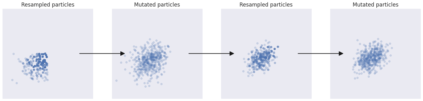
The population progressed much faster towards the target distribution.
Summary #
To summarize, here is the basic SMC algorithm again:
# hyperparameters
n_particles = 2000
n_steps = 10

# initialize population of particles from prior
particles = sample_prior(n_particles)
# main loop
for step in range(n_steps):
    # compute particle weights in proportion
    # to the posterior distribution probability
    weights = compute_weights(particles, posterior)
    # resample particles (with replacement)
    # based on their weights
    particles = resample(particles, weights)
    # mutate particles to reintroduce variation
    # and better explore the posterior distribution
    particles = mutate(particles)
# final approximation is given by the final particles
posterior = particles
What about the prior? #
You might have noticed a large repetition of the word “posterior”, and a strange absence of “prior”. To keep things simple I chose to work with an implicitly uniform prior which does not affect the posterior calculations. Indeed the two are needed for a complete Bayesian inference. And in fact there is something very interesting that can be done when combining the two into a general SMC algorithm. That’s the topic of the [next article]!